Introduction to LOFAR data processing

Introduction to LOFAR data processing
Harish Vedantham
Netherlands Institute for Radio Astronomy
University of Groningen

These are my notes from a LOFAR data processing tutorial I gave to students in Sofia, Bulgaria between May 22 and May 26 of 2023. The school was organised by the STELLAR project. If you are already familiar with radio interferometry, then you can just follow the blue text and the code blocks. Else you may want to read the whole thing to get some background information on the motivation for the different steps we will be following.
Note that these are the notes I made as I was preparing for the lectures and tutorials. So it is not a polished end product but it is good enough for someone with a bit of grit and motivation to come up to speed with basic LOFAR data reduction.
There are other more polished and more comprehensive material out there, the foremost of which is the LOFAR imaging cookbook.
The only advantage of following what I have written here is that I provide some background information motivating the various steps which may be useful for a beginning student of interferometry.
Finally, I must note that what follows is not the “black-belt” way to reduce LOFAR data. I deliberately made this choice so that the student is not lost in all the excruciating details that one must get just right to get the best image from a complex telescope such as LOFAR. Instead I wanted the students to focus on understanding the basic steps of the data reduction which essentially meant I need to follow the simplest path from data to a “good enough” image. In any case, the black belters have written pipelines which work off the shelf (more of less!). Examples are LINC and KillMS + DDFacet. LINC particularly has some good documentation and support for bug notifications etc.
Singularity image
We will be using a singularity “image” which has all the necessary software within. You can think of singularity as a software container that has all the software including an operating system within it. That way you do not have to spend time installing all the software. You just need to get the singularity file and open it with the command singularity. It’s a really clever way to make important software portable across different computing systems.
So to download the LINC (name of the pipeline code that we use to process LOFAR data) you just have to run
singularity pull docker://astronrd/linc
It will then do a bunch of things and leave you with the singularity image in a file called
linc_latest.sif
That’s it, you have all the software necessary to process LOFAR data!
You can now use this via two routes.
One option is to simply run an executable file within the container by saying
singularity exec [exec options…] <container_file_name> <command_to_excecute>
Or you can enter to a linux shell inside the container by saying
singularity shell <container_file_name>
There is one important thing here. You need to make sure that you can access the file system from inside the container. This does not happen by default. Instead you have to tell singularity that you want this.
So for example, you can do
singularity shell -B /home/harish/lofar_tutorial/ linc_latest.sif
Voila. You now have a linux prompt with all the software installed!
Data format
LOFAR data is stored in a standard format called “Measurement Set”.
You can find the format specification here
But essentially it is a bunch of tables each having with rows and columns with information.
The “MAIN” table is where the interferometric data is.
You can think of each row as a “measurement”.
The columns have the actual data, the time at which the data were taken, the names of the two antennas that formed the baseline etc.
You can open a Measurement set with the python wrapper to the casacore libraries that were written in C++ to access and manipulate measurement set data. The python wrapper is called python-casacore and can be found here .
Here is an example where I open a measurement set’s main table
$ python3
>>> msname = “L196867_SAP000_SB000_uv.MS.5ch4s.dppp”
>>> from casacore.tables import table
>>> t = table(msname,readonly=True)
Successful readonly open of default-locked table L196867_SAP000_SB000_uv.MS.5ch4s.dppp: 26 columns, 10532529 rows
>>>
Ok good. So the table is open. You can see that it has 26 columns and over 10 million rows!
Let us see what the columns are
>>>t.colnames()
[‘UVW’, ‘FLAG_CATEGORY’, ‘WEIGHT’, ‘SIGMA’, ‘ANTENNA1’, ‘ANTENNA2’, ‘ARRAY_ID’, ‘DATA_DESC_ID’, ‘EXPOSURE’, ‘FEED1’, ‘FEED2’, ‘FIELD_ID’, ‘FLAG_ROW’, ‘INTERVAL’, ‘OBSERVATION_ID’, ‘PROCESSOR_ID’, ‘SCAN_NUMBER’, ‘STATE_ID’, ‘TIME’, ‘TIME_CENTROID’, ‘DATA’, ‘FLAG’, ‘LOFAR_FULL_RES_FLAG’, ‘WEIGHT_SPECTRUM’, ‘CORRECTED_DATA’, ‘MODEL_DATA’]
It is good to introduce some of the columns here
UVW has the baseline vector information. For example let us check the baseline at the i = 10 row number.
>>> t[10][‘UVW’]
array([347.8941652 , 393.02896846, 72.86538322])
Those are the x,y, and z components of the baseline vector whose data is in that particular row.
ANTENNA1 and ANTENNA2 have the id’s of the antenna that make up the baseline.
For example
>>> t[10][‘ANTENNA1’]
0
>>> t[10][‘ANTENNA2’]
4
So this baseline has been formed between antennas 0 and 4.
Note that there is a separate antenna table which has all the information about the antennas (their location, type etc.)
TIME columns has the time at which the visibilities in this row were measured
For example
>>> t[10][‘TIME’]
4895244222.002781
This is in units of second. So if you divide that by 3600*24 you get 56657.919236143294 which is the MJD value (Modified Julian Day). This happens to correspond to Dec 31st in 2013.
Ok now the visibility data of course in the DATA columns. Let us see what that looks like
>>> t[10][‘DATA’]
array([[ 1.4692880e-04-5.0897197e-06j, 2.0738231e-05-9.1280635e-06j,
-9.1629026e-06-1.0781963e-05j, 1.4645154e-04+5.8871698e-05j],
[ 1.5119652e-04+9.9043973e-06j, 1.4225746e-05+1.0215125e-06j,
-2.2907270e-05+2.2927508e-05j, 1.4993091e-04+4.9046266e-05j],
[ 1.6090520e-04-4.5281781e-06j, 1.0693016e-06-9.9634372e-06j,
1.8860512e-05+1.7586775e-05j, 1.6076493e-04+3.7567075e-05j],
[ 1.3379545e-04+8.7470880e-06j, 1.1277861e-05+1.7836361e-05j,
3.8624198e-06+3.6346677e-07j, 1.5921239e-04+4.2929260e-05j],
[ 1.5956792e-04-1.3678416e-05j, 2.2152251e-05+2.1676595e-05j,
2.8818265e-05-1.6163740e-06j, 1.6466140e-04+5.8218047e-05j]],
dtype=complex64)
As you can see, the visibility data is a complex quantity with real and imaginary parts. What you have here is a 5 X 4 matrix of complex numbers.
What are these dimensions? The 5 is along frequency and the 4 is along polarisation. This means that there are 5 frequency channels over which the visibilities have been measured. Their frequency values are are in another table!
There are 4 polarisation products which in case of LOFAR correspond to XX, XY. YX and YY dipole-dipole correlations.
What about the columns that are called MODEL_DATA and CORRECTED_DATA
Well these are also visibility DATA. MODEL_DATA holds the visibilities for the best model of the sky you have at the moment. That is, these are what you think the visibilities ought to look like if the model of the sky you have is perfect. CORRECTED_DATA is the DATA that has been calibrated, that is the instrumental response has been removed and it ideally represents the “true” visibilities you get from the sky.
If your calibration is perfect and your sky model is perfect, then MODEL_DATA will be equal to CORRECTED_DATA.
As you will see later, calibration is usually an iterative process. You calibrate, make an image and use that image to make a model of the sky. Then you assume that this model represents the truth and again find the calibration solutions that bring your corrected data as close to the model data as possible. With the new solutions, you make another image. From that image you build another model and so on until hopefully the process converges.
Ok now let us have a look at the FLAG column.
>>> t[10][‘FLAG’]
array([[False, False, False, False],
[False, False, False, False],
[False, False, False, False],
[False, False, False, False],
[False, False, False, False]])
The FLAG data has the same dimension (5 X 4) as the visibility data. These are the boolean flag values for each visibility complex number we have. Here all of them are False which means that this data has not been flagged as corrupted by interference.
Finally, what are the 10 million+ rows for?
Well we just had a look at row number 10. Each row has a unique time, and antenna pair. So nrows is just the number of antenna pairs we have data on times the number of time-steps.
But how many antennas do we have in this observations. For that we can open the ANTENNA table which is in the main measurement set directory. So you can do
>>> from casacore.tables import table
>>> t = table(“L196867_SAP000_SB000_uv.MS.5ch4s.dppp/ANTENNA”)
>>> t.nrows()
62
Ah, so we have 62 antennas. The number of unique baselines is then 62*(62-1)/2 = 1891 and then we have 62 autocorrelations. So there will be 1953 unique baselines.
Note that not all baselines may be available always but the standard LOFAR measurement set will typically have all of the baselines in it.
So the main measurement set table has the following row format
time index = 0, baseline index = 0
time index = 0, baseline index = 1
……
time index = 0, baseline index = 1952
time index = 1, baseline index = 0
time index = 1, baseline index = 1
….
and so on.
Now that the ANTENNA table is already open, let us see what else it has
>>> t.colnames()
[‘OFFSET’, ‘POSITION’, ‘TYPE’, ‘DISH_DIAMETER’, ‘FLAG_ROW’, ‘MOUNT’, ‘NAME’, ‘STATION’, ‘LOFAR_STATION_ID’, ‘LOFAR_PHASE_REFERENCE’]
Let us see what values they have for the i = 0th antenna
>>> t[0]
{‘OFFSET’: array([0., 0., 0.]), ‘POSITION’: array([3826896.235, 460979.455, 5064658.203]), ‘TYPE’: ‘GROUND-BASED’, ‘DISH_DIAMETER’: 31.262533139844095, ‘FLAG_ROW’: False, ‘MOUNT’: ‘X-Y’, ‘NAME’: ‘CS001HBA0’, ‘STATION’: ‘LOFAR’, ‘LOFAR_STATION_ID’: 0, ‘LOFAR_PHASE_REFERENCE’: array([3826896.235, 460979.455, 5064658.203])}
Ah, so it has all the details you may need about the antenna like its location, type of polarisation, name etc.
Now that you have the hang of it, you can explore other tables within the main measurement set. For example the SPECTRAL_WINDOW table has all the information about the frequency setup such as the centre frequency of the channels etc.
There are many more tables which ensure that all the information that may be necessary to process the data is available.
Just ls the measurement set and you will see what all tables it has
ls ../data/L196867_SAP000_SB000_uv.MS.5ch4s.dppp
ANTENNA OBSERVATION STATE table.f2_TSM0 table.f7
DATA_DESCRIPTION POINTING solutions.h5 table.f3 table.f7_TSM0
FEED POLARIZATION solutions.h5_copy table.f3_TSM0 table.f8
FIELD PROCESSOR solutions.h5_copy_copy.h5 table.f4 table.f8_TSM0
FLAG_CMD QUALITY_BASELINE_STATISTIC table.dat table.f4_TSM0 table.info
HISTORY QUALITY_FREQUENCY_STATISTIC table.f0 table.f5 table.lock
LOFAR_ANTENNA_FIELD QUALITY_KIND_NAME table.f1 table.f5_TSM0
LOFAR_ELEMENT_FAILURE QUALITY_TIME_STATISTIC table.f1i table.f6
LOFAR_STATION SPECTRAL_WINDOW
In practice, you will seldom access the visibilities at this low level unless you get into the art and science of writing data processing code.
Most telescopes will have these data processing code already developed. So you can use these software tools to write a high-level algorithm to process the data without worrying about the nitty-gritty details at the individual visibility level.
But it is always good to know what is under the hood!
Finally, the singularity image has a nice command called msoverview which will open some of the sub-tables and print out important details about a given measurement set. For example.
Singularity> msoverview in=L196867_SAP000_SB150_uv.MS.5ch4s.dppp
msoverview: Version 20110407GvD
2023-05-18 18:51:31 INFO MSMetaData::_computeScanAndSubScanProperties Computing scan and subscan properties…
================================================================================
MeasurementSet Name: /home/harish/lofar_tutorial/data/L196867_SAP000_SB150_uv.MS.5ch4s.dppp MS Version 2
================================================================================
10
Observer: unknown Project: LC1_039
Observation: LOFAR
Antenna-set: HBA_DUAL_INNER
10
Data records: 10532529 Total elapsed time = 21602 seconds
Observed from 31-Dec-2013/22:03:40.0 to 01-Jan-2014/04:03:42.0 (UTC)
10
Fields: 1
ID Code Name RA Decl Epoch nRows
0 BEAM_0 08:13:36.067800 +48.13.02.58100 J2000 10532529
10
Spectral Windows: (1 unique spectral windows and 1 unique polarization setups)
SpwID Name #Chans Frame Ch0(MHz) ChanWid(kHz) TotBW(kHz) CtrFreq(MHz) Corrs
0 SB-150 5 TOPO 144.261 36.621 183.1 144.3344 XX XY YX YY
Typical steps & DP3
There is no universal set of steps in a radio interferometric pipeline but the usual steps are as follows. Each pipeline will have some combination of the steps we will now discuss. You will typically write a script that will concatenate these steps in some order and with some input parameters to process the data.
To write such a script, you will need a higher level interface. The currently most common package that provides this interface and all the code that does the real work is called CASA, short for Common Astronomy Software Applications.
While CASA works perfectly well for processing data from many radio interferometers, we cannot use this for LOFAR due to the sheer complexity of the LOFAR calibration and data volume challenge.
So an entire separate package had to be written. This is called DPPP or DP3 which is short for Default Pre-Processing Pipeline
DP3 is run from the command line using
$ DP3 <parset-file-name>
where the parset file has all the information about what the pipeline must do.
Here is the simplest parset file I can think of
msin = L196867_SAP000_SB000_uv.MS.5ch4s.dppp
msout = new_copy.MS
steps=[]
This just instructs DP3 to take the measuremet set specified by msin and write the output to a new measurement set whose name is specified with msout.
And there are no steps to perform!
You write your pipeline by giving it a series of steps using, for example.
steps = [flag, average, calibrate]
and the rest of the parset file will have to describe the parameters for each step (for example, how much should DP3 average along the time and frequency axis) etc.
Writing a pipeline
Staging
Usually the data you want to process is archived in some data centre (radio data now-a-days are too big to carry around in your laptop).
The data centre will have some Web-interface where you can login and search for your data. For example, LOFAR data is archived in the LOFAR Long Term Storage
Once you have located your data you can “stage” it which means that the data centre loads the data on to hard drives on a machine that has read access opened to the outside world. You will then be given instructions on how to download this data. Similar setups are in place for all large telescopes such as the JVLA and GMRT.
For the sake of this tutorial, to speed things up, the data you will use are already staged and downloaded.
Flagging
This is the step where unwanted human generated interference (RFI) is “flagged”
By flagged we mean that we do not remove the contaminated data. We merely set a “flag” so that we discard this data in other steps.
A flagger software will set these flags for you. LOFAR uses a flagger called AOflagger written by Andre Offringa.
Like other flaggers AOflagger will go baseline by baseline and examine the visibility data in the time-frequency plane to find fingerprints of interference. Usually this fingerprint is defined as anything that is very narrow in time or in frequency or both. The vast majority of astrophysical signals will be broad in time and in frequency. Therefore the software will only plants “flags” on data that it thinks are contaminated.
As explained below, in order to keep the data size manageable, in this tutorial the initial flagging step has already been performed.
As future reference, here is an example DP3 parset which calls AOflagger to run on your measurement set (Note that this step does not require you to write to a new measurement set)
msin = L196867_SAP000_SB000_uv.MS.5ch4s.dppp
steps=[flag]
flag.type = aoflagger
flag.memoryperc = 20
Here the flagger is restricted to use no more than 20% of the available RAM memory. Note that the larger this value is, the better because the flagger can work on a larger chunk of data which will allow it to better discriminate things that are varying rapidly with time (interference) from things that are varying smoothly with time (astrophysical signal).
There are other optical parameters that can be specified to “tune” the flagger to the data in question which can be found in the DP3 reference manual.
Averaging
This step essentially averages data along time and/or frequency axis. This is mainly used to reduce the size of the data so it is easy to handle given the computing resources you have.
The raw data of LOFAR can be tens of terabyte in volume for several hours of observations. This “Raw” data that comes out of the correlator typically has a time resolution of 1second or 2 seconds and a frequency resolution of a few kiloHertz. Most astrophysical signals are constant over this time-frequency interval so there is virtually no loss of astrophysical information by averaging down to say 10 seconds and 1 MegaHertz.
There is a penalty you pay by averaging however. Nothing comes for free!
(1) Averaging reduces the effective field of view of your instrument. This is because sources that are away from the pointing centre will have visibilities that vary more rapidly in time and frequency. And if you average too much along time and frequency, you will eliminate this information making the source “invisible” in your final image.
(2) Averaging can corrupt otherwise fine data if you are not careful. Let us say you are averaging 10 steps in time. Essentially you will average ten numbers to output one number. Let us say one of the ten value is corrupted (due to interference, or bad calibration etc.). In the original data, if you can identify the bad sample, you can reject it. But in the averaged data, this is not possible. Therefore we always run a flagging step before averaging. That way flagged data are not taken in during the average step.
For obvious reasons, averaging essentially requires you to write your averaged data into a new measurement set. Else we will be adding duplicate data to the measurement set and the data and flag column entries will have heterogeneous data types.
The initial averaging step has also been already performed for this tutorial. This is because the native resolution at which LOFAR typically acquires data leads to very large data sets. We acquire data at this fine resolution so we can identify interference effectively with minimal data loss and then average down to manageable size. But we don’t have enough storage on the machine we are using to have the original data.
For reference, here is an example averaging parset
msin = L196867_SAP000_SB000_uv.MS.16ch1s.dppp
msout = L196867_SAP000_SB000_uv.MS.2ch4s.dppp
steps = [avg]
avg.type = average
avg.timestep = 4
avg.freqstep = 8
This will average the data down 4 times in time and 8 times in frequency. So the output data will be 8 X 4 = 32 times smaller in size!
Calibration
Now we get to the most interesting part of the tutorial, where we will calibrate the data. Calibration is necessary because the electronics and antenna are not ideal elements; they have a response function which needs to be removed to get to the true “visibilities”.
Typically there are a few types of errors that need to be calibrated as explained below and depicted in the sketch here:
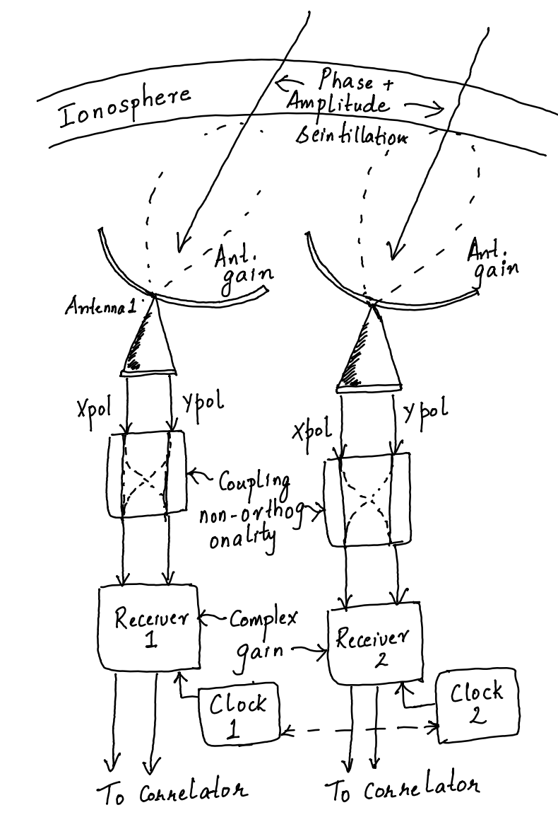
(1) Ionospheric phase: The radio waves we receive must pass through the Earth’s ionosphere which introduces a frequency dependent delay. This value of delay can vary from location to location and with time. If these delays are not corrected for then the images will be fuzzy and the source locations may also not be accurate. Ionospheric effects become worse at lower frequencies. A general rule of thumb is that you should pay attention to this effect if your frequency is below ~ 1 GHz and pay very close attention if your frequency is below 300 MHz.
(2) Polarised antenna response : The antenna has a gain that is not isotropic. That is to say signals from some directions induce a response in the electronics that is different from the response induced by the same strength signal from another direction. This has to be corrected for to get at the “true” signal strength. More over the LOFAR antennas are collect signals on two polarisations which may not be perfectly orthogonal. Also the signal from one antenna may couple to the other. These effects need to be modelled and removed from the data.
(3) Electronic gain: The antenna is connected to amplifiers, filters and mixer circuitry which have their own complex response (amplitude and phase) with which they modulate the signal. This again has to be modelled and removed. In addition, all the antenna elements of an interferometer must be on the same time/frequency standard. That will be the case if they are connected to the same “clock” source but this is often not the case. In LOFAR, the “core stations” are on a common clock but the Dutch “remote stations” and the “international stations” are on a their own clock sources. Hence one must synchronize all of these stations to a common standard. This is particularly important for interferometry because delay is how an interferometer measures the locations of the source on the sky accurately and delay can only be accurately measured if the two ends of an interferometer are on a common clock.
The way interferometer are calibrated is typically as follows: We observe a reasonably bright source whose position on the sky, brightness and structure are very well known. We then know what the visibilities should look like (Called model visibilities which have their own column in the measurement set). Then we find the “complex antenna based gains” that when applied to the actual data will bring it close to the model visibilities modulo any thermal noise that will be present. This is a high dimensional non-linear optimization process that is algorithmically very complex. Luckily all of this software has been written for us (within DP3) and it works quite well in most circumstances.
Another point worth noting here is that we often do not have enough constraints in the calibration to solve for everything. So we need to make some compromises. For example a common assumption is that the complex gain of each antenna element which incorporates all the above errors is a separable function in time and frequency. This is to say that we can independently solve for how to gain varies in frequency and then independently solve for how it varies in time. We multiply the two effects to get the complex gain of the antennas in the time-frequency plane.
So you will hear of a separate bandpass calibration in many interferometry pipelines.
Anyways, getting back to the LOFAR data at hand. The first step in the calibration process is to get a skymodel.
DP3 again has a format which it recognises. I have chosen the dataset we are processing to have a bright source in the centre of the field called 3C196. You can find the basic properties of the source here.
Here is the model for the central bright source which will use for calibration.
# (Name, Type, Ra, Dec, I, Q, U, V, ReferenceFrequency=’150.e6′, SpectralIndex, MajorAxis, MinorAxis, Orientation) = format
3C196_0, GAUSSIAN, 08:13:35.925, 48.13.00.061, 33.5514, 0, 0, 0, 1.5e+08, [-0.572, -0.042], 1.476, 1.091, 135.27
3C196_1, GAUSSIAN, 08:13:35.772, 48.13.02.507, 12.3129, 0, 0, 0, 1.5e+08, [-0.973, -0.319], 2.738, 1.754, 93.3
3C196_2, GAUSSIAN, 08:13:36.182, 48.13.04.725, 14.603, 0, 0, 0, 1.5e+08, [-0.557, -0.27], 1.034, 0.248, 124.03
3C196_3, GAUSSIAN, 08:13:36.389, 48.13.02.735, 22.6653, 0, 0, 0, 1.5e+08, [-0.84, -0.288], 1.456, 2.159, 324.58
As you can see the source is modelled as a set of 4 Gaussians which is a close approximation to what the source really looks like.
Here is an old image of 3C196 made by Lonsdale and Morrison (1983)
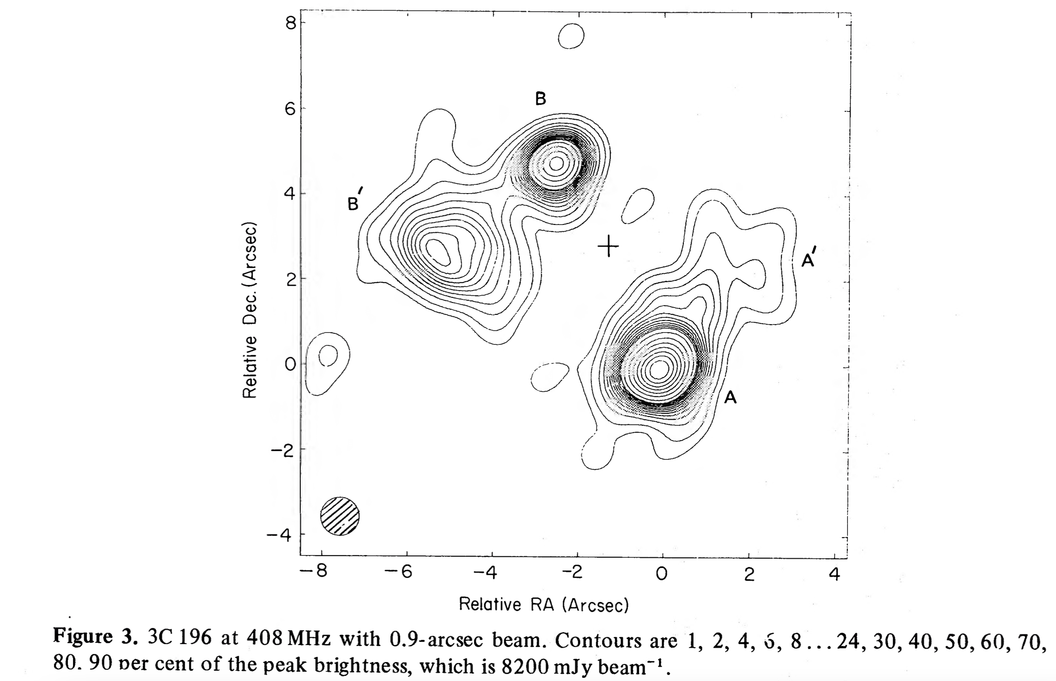
See it does look like for different semi-Gaussian components!
We then have to use a command to convert this text file which is human readable into a format that the calibration software understands. This command is called makesourcedb and it understands that the first line of the ascii file that starts with a # is specifying the format in which the source model is specified by subsequent lines.
You use it as follows
$ makesourcedb in=<ascii-file-name> out=<sourcedb-file-name>
Now you have all that you need to run a calibration using DP3.
There are two tasks in DP3 to calibrate: gaincal and ddecal. The difference between the two is that gaincal is used for direction independent gains and ddecal is used for direction dependent gains. In other words there are gains that depend on direction on the sky such as ionospheric phase and antenna beam gain. Then there are gain terms that do not depend on sky direction such as the gains of the electronics in the receiver.
Traditional radio telescopes had very small fields of view and used dish antennas. LOFAR on the other hand has a large field of view (16 sq degrees at 150 MHz) and uses electronic beam steering. These two differences makes it necessary to use direction dependent calibration to achieve the full potential of the system.
Let us run a gaincal on our data. Here is an example parset file
msin = ../data/L196867_SAP000_SB000_uv.MS.5ch4s.dppp
msin.datacolumn = DATA
msout=.
steps = [cal]
cal.type = gaincal
cal.caltype = fulljones
cal.parmdb = fulljones.h5
cal.uvlambdamin = 20
cal.solint = 1
cal.nchan = 1
cal.propagatesolutions = True
cal.usebeammodel = False
cal.sourcedb = 3c196_4comp_model.sourcedb
As you see, there is just one step to perform which is “Cal” of type “gaincal“
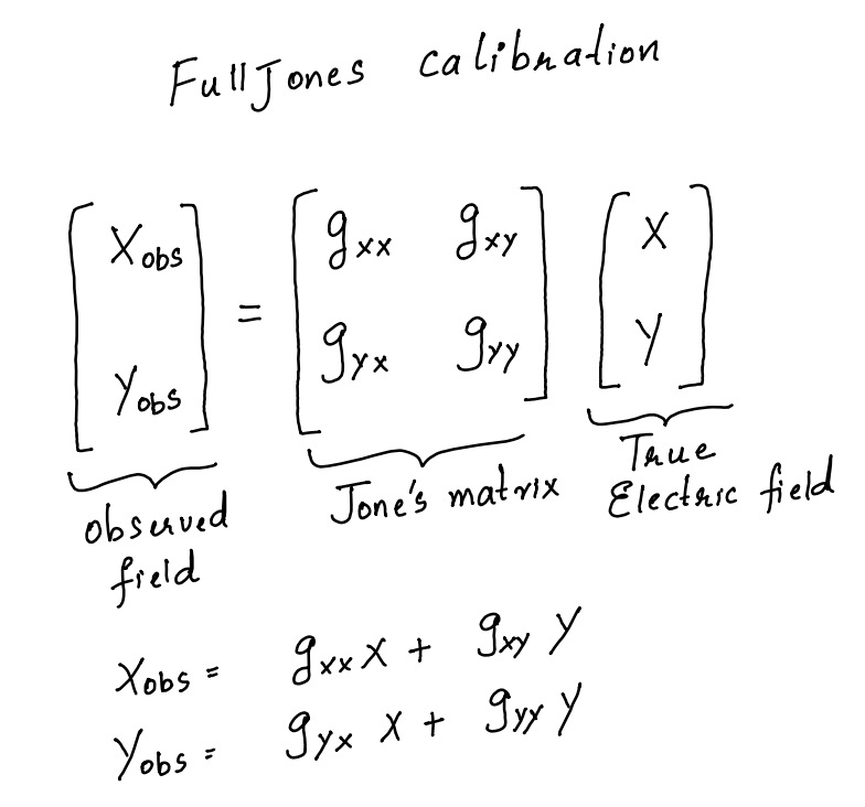
The type of calibration here is “fulljones” which means that the entire Jone’s matrix will be solved for (see image below) for each antenna.
One can also solve for only the diagonal elements (see image below)
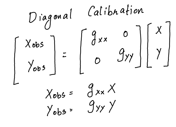
Note that the gains are complex quantities. So one can also solve for only their amplitudes or phases.
uvlambdamin is to exclude the shortest baselines from calibration. This is done because the shortest baselines can have worse quality data mainly because they tend to be sensitive to large-scale brightness variations on the sky (remember that short baselines measure large angular scales and long baselines measure small angular scale features) which is not part of our model of 3C196 that is we have not included in our model, the diffuse radio emission from our Galaxy. So to not let this omission lead to errors, we must exclude the shortest baselines.
solint and nchan decide the cadence of the solutions. Here both are set to 1 which means that each timestep and each channel in the visibility will get its own solution (for each antenna of course). This is possible because we have a very bright source in our pointing centre (3C196) which ensures that there is enough signal versus noise for us to solve for each time and frequency step.
If this is not the case, then one will choose large enough values of solint and nchan so that there is enough signal-to-noise ratio for a solution.
The usual rule of thumb is that the calibrator must be detected with a signal to noise ratio of at least 3 (and ideally 5) on a single baseline within the solution interval in time and frequency.
Checking the solutions
It is always a good idea to check the calibration solutions, i.e. the complex gains per antenna, time, and frequency.
The solutions are stored in a file format called Hierarchical File Format
There is a software package called LOFAR Solution Tool or LoSoTo which has been written to manipulate (for e.g. interpolate) and plot calibration solutions. So one option is to use this package to plot the solutions for inspection.
An easier way for those of us who are used to python is to use a python package called lofar-h5parm that can do the plots in an interactive way.
I have made a singularity image for this so we don’t have to spend time with installations.
You can find the singularity recipe here
Once you have entered this container you can just say
h5plot <h5 file name>
and it will open an interactive screen where you can select the gains you want to plot.
In general you are looking to see if the calibration operations has worked well. How do you make sure of that?
Some basic sanity checks you can do are
(1) The gains should be varying smoothly with time and frequency. This is because all the effects we are trying to calibrate will vary slowly over frequency. For example the ionospheric phase is proportional to 1/frequency. Any clock offset will give rise to a phase that varies linearly with frequency. Similarly electronic components gains vary over many Megahertz-scales at 150 MHz.
(2) The XX and YY phases should (roughly speaking) track one another. This is because the ionosphere will induce nearly the same phase shifts on the X and Y hands. The electronic gains vary usually due to temperature changes etc which should be to first order common for the two polarisations.
(3) The core station phases should be close to zero whereas the remote station phases can vary by > 2*pi on timescales of tens of seconds. This is because all core stations are on a common clock, whereas remote stations are not. So drifts in the remote stations clocks will show up as phase variations.
(4) the variations in the gains should be roughly what one would expect from the signal to noise ratio of the source using which calibration was done. This is a bit harder to calculate but a rough rule of thumb is that the fractional variation should be roughly equal to 1/SNR.
Applying the solutions
Once we are satisfied that the solutions are fine. We will apply the solutions. This can be done via DP3 using the applycal step. An example parset is shown below
msin = ../data/L196867_SAP000_SB000_uv.MS.5ch4s.dppp
msin.datacolumn=DATA
msout=.
msout.datacolumn=CORRECTED_DATA
steps = [apply]
apply.type = applycal
apply.parmdb = fulljones.h5
apply.correction=fulljones
Here we are saying that we should apply the calibration solutions in the file fulljones.h5 to the visibilities and write the resulting visibilities into the CORRECTED_DATA column.
Imaging
Now we are finally ready to make an image with the calibrated data (the moment of truth where you know how well the preceding steps have worked)
Imaging has there main steps
(1) Gridding: All the visibilities selected for imaging are gridded on to a regular 2D grid on the uv-plane (also called the Fourier plane)
(2) Making the “dirty” image: The gridded visibilities are inverse Fourier transformed to get an image. However interferometers usually have bad point spread function (i.e. high sidelobe level) so the image will be a jumble of sidelobes of all the sources in the field.
(3) Cleaning: This is an interative procedure where we try to remove the sidelobes of the point spread function to get a “clean” image.
Usually, the three steps are not performed sequentially at once. Rather the algorithms tries to clean in the Fourier domain (uv-plane) so the iterative procedure usually loops through steps 2 and 3 above.
Interferometric imaging is quite complex especially if the field of view of the instrument is large and we have a separate software package to do this task calledwsclean.
Imaging has a lot of parameters which cannot all be covered here. The important ones as as follows:
(1) uvmax and uvmin: These are used to make cuts in the uv-plane within which data are used in the imaging process. The uvmin cut if used to get rid of very short baselines that are very sensitive to large scale diffuse emission (in case we are not interested in it) and also because the shortest baselines also tend to be the most affected by interference (this is because interference is locally generated so short baselines “see” the same interference signals).
(2) scale: This is used to set the pixel size in the image. 1/uvmax is the angular resolution (in radian!) of the data, so you want the pixel size to be less than this value else you will “under sample” the image. Theoretically speaking 1/2 of 1/uvmax is sufficient image scale according to the Nyquirst theorem (remember that the uv and image planes are Fourier transforms of one another). But in practice we choose a value that is 1/3 of 1/uvmax or more preferably 1/4 of 1/uvmax as the image resolution.
(3) Weighting: This parameter is used to decide the relative importance that we wish to give one visibility versus another. The best signal to noise ratio is produced when all visibilities (with the same noise) are given the same weight. But this is not always desirable. This is because most interferometers tend to have many more small baselines compared to long baselines. Also the baseline distribution may not be very smooth across the uv-plane. This non-smoothness tend to generate a point spread function that has a high sidelobe level. In addition, small baselines also have worse angular resolution and you may be interested in resolving sources instead of diffuse emission. In these cases one may use “uniform” weights. By this we means that each cell in the uv-plane is given the same weight regardless of how many visibilities fall into it. This will create a point spread function that is narrower (so better angular resolution) but an image with worse signal to noise ratio. Of course we can also have a middle-ground with an adjustable scale to go from natural to uniform weights. This is typically called robust weighting with a parameter that sets the location on this adjustable scale.
Then there are a few critical parameters related to cleaning the image of the sidelobes of the point spread function. Cleaning is an iterative process so the gain in each iteration must be set. You can think of the gain as the fraction of the sources that is “cleaned” in each iteration. Having a high gain means that cleaning will be faster but it will have a higher chance of making mistakes (i.e picking up sources that are not real but rather due to sidelobes of other sources). Of course picking a small gain means that cleaning will be slower as more iterations are necessary to converge to the final clean image. The general rule of thumb is to use a gain of 0.1 which is to say that in each iteration must clean 10% of the flux of the brightest source in that iteration.
An example wsclean imaging command is given below. Note that this is quite a minimalist command and wsclean has many more options to obtain the best possible image given the data quality and also to enhance speed via parallel computation.
$wsclean -minuvw-m 200 -maxuvw-m 90000 \
-size 7500 7500 \
-weight briggs -0.5 \
-data-column CORRECTED_DATA \
-pol i \
-name test \
-scale 1.5arcsec \
-niter 10000 \
../data/L196867_SAP000_SB000_uv.MS.5ch4s.dppp
Here we have chosen a max uv length of 90k metres which at a wavelength of 2m will be 45k lambda. This should give a PSF no narrower than 1/45k radian = 4.6 arcsecond. So we have chosen an image scale of 1.5 arcsecond.
The image will have 7500 x 7500 pixels which means the field of view has a width of 7500 pixel * 1.5 arcsec/pixel = 3.125 degree. The LOFAR single stations have a diameter of 30m which is around 15 lambda. Their field of view is therefore 1/15 radian = 3.8 degrees. So we are imaging a large fraction of the field of view.
The number of iterations is chosen to a large value, although the algorithm will stop cleaning when it has reached the noise in the image.
Writing a script
We do not wish to manually process each sub-band file, So we will have to write a script
Fortunately this is quite simple to do in bash (you could also do this in python).
Here is a simple bash script to process a series of measurement sets one after the other
#!/bin/bash
for i in {000..165..15}; do
msname=`echo -n ../data/L196867_SAP000_SB${i}_uv.MS.5ch4s.dppp`
echo $msname
DP3 calibrate.parset msin=$msname cal.parmdb=$msname/fulljones.h5
DP3 applycal.parset msin=$msname apply.parmdb=$msname/fulljones.h5
done
Which I hope is self explanatory.
As for the imaging step, we need to combine all the MS into a single image.
So we would say something like
wsclean \
-minuvw-m 200 \
-maxuvw-m 90000 \
-reorder \
-j 3 \
-size 7500 7500 \
-weight briggs -0.5 \
-data-column CORRECTED_DATA \
-pol i \
-name test \
-scale 1.5arcsec \
-niter 10000 \
-mgain 0.8 \
-parallel-gridding 4 \
-parallel-reordering 4 \
../data/L196867_SAP000_SB000_uv.MS.5ch4s.dppp ../data/L196867_SAP000_SB015_uv.MS.5ch4s.dppp ../data/L196867_SAP000_SB030_uv.MS.5ch4s.dppp ../data/L196867_SAP000_SB045_uv.MS.5ch4s.dppp ../data/L196867_SAP000_SB060_uv.MS.5ch4s.dppp ../data/L196867_SAP000_SB075_uv.MS.5ch4s.dppp ../data/L196867_SAP000_SB090_uv.MS.5ch4s.dppp ../data/L196867_SAP000_SB105_uv.MS.5ch4s.dppp ../data/L196867_SAP000_SB120_uv.MS.5ch4s.dppp ../data/L196867_SAP000_SB135_uv.MS.5ch4s.dppp ../data/L196867_SAP000_SB150_uv.MS.5ch4s.dppp ../data/L196867_SAP000_SB165_uv.MS.5ch4s.dppp
It is nice that wsclean lets to list a number of measurement sets to be jointly imaged.
Perusing the image
There are a few softwares that can display standard format astronomical images. A common one is called ds9
It has an interface that is quite easy to use and it has the usual functionality to zoom, pan, change colorscales, annotate and do some basic statistics on the image
The first thing we should check in the image is its quality. We see that 3C196 (the bright central source) has artefacts around it that run throughout the image. This shows that our calibration has not been perfect. What is the rms level of these artefacts? If we use the ds9 region–> analysis we find that it is around 1.5 mJy. This means that away from 3C196, the image has a dynamic range of 70 Jy / 1.5 mJy = approx 47,000. This is quite good for a first image!
What about the thermal noise in the image? One way to check this is to make a Stokes V image of the sky which is virtually devoid of sources (assume this for now) which means the image must just have noise in it. Our Stokes V image has an rms noise of 0.33 mJy so we are off by a factor of 4.5 from thermal noise. This is quite common in areas of the sky that have a super-brigt source in them (3C196 in our case) and our Stokes I images are limited bu dynamic range rather than thermal noise.
Here is a screenshot of our Stokes-I (left) and Stokes-V (right) images.

Introduction to LOFAR data processing Tutorial